
FIR filter design with Python and SciPy
Author: Matti Pastell
Tags:
SciPy, Python, DSP
Jan 18 2010
SciPy really has good capabilities for DSP, but the filter design functions lack good examples. A while back I wrote about IIR filter design with SciPy. Today I’m going to implement lowpass, highpass and bandpass example for FIR filters. We use the same functions (mfreqz and impz, shown in the end of this post as well) as in the previous post to get the frequency, phase, impulse and step responses. You can download this example along with the functions here FIR_design.py. To begin with we’ll import pylab and scipy.signal:
from pylab import *
import scipy.signal as signal
Lowpass FIR filter
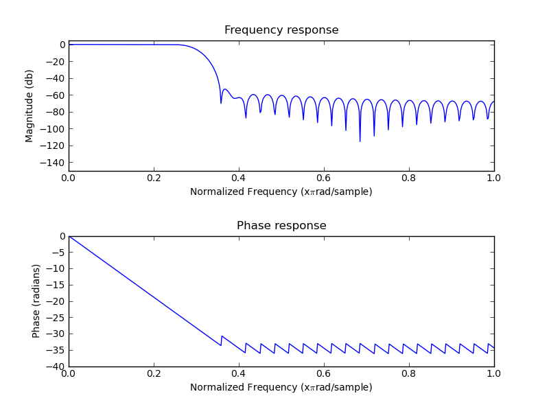
Designing a lowpass FIR filter is very simple to do with SciPy, all you need to do is to define the window length, cut off frequency and the window:
n = 61
a = signal.firwin(n, cutoff = 0.3, window = "hamming")
#Frequency and phase response
mfreqz(a)
show()
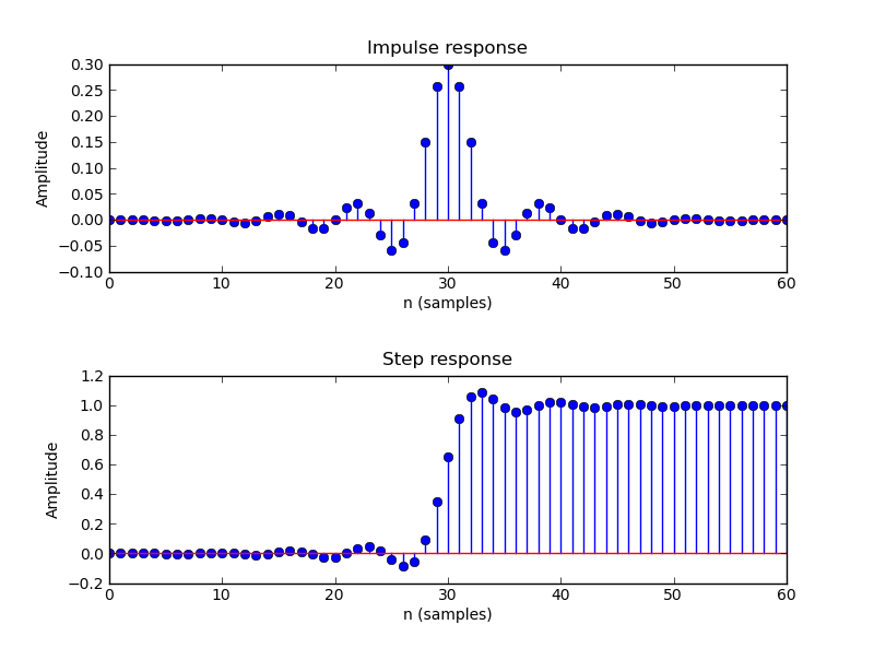
#Impulse and step response
figure(2)
impz(a)
show()Which yields:
Highpass FIR Filter
SciPy does not have a function for directly designing a highpass FIR filter, however it is fairly easy design a lowpass filter and use spectral inversion to convert it to highpass. See e.g Chp 16 of The Scientist and Engineer’s Guide to Digital Signal Processing for the theory, the last page has an example code.
n = 101
a = signal.firwin(n, cutoff = 0.3, window = "hanning")
#Spectral inversion
a = -a
a[n/2] = a[n/2] + 1
mfreqz(a)
show()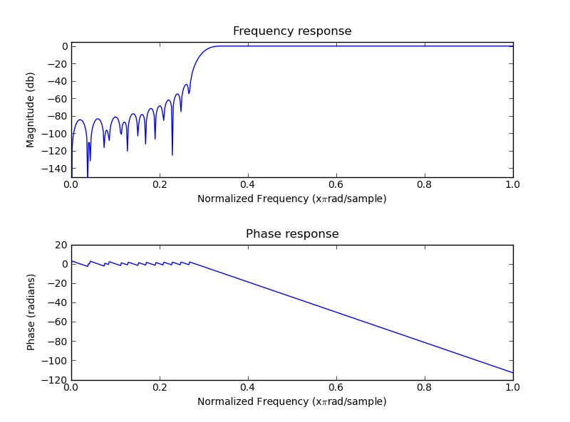
Bandpass FIR filter
To get a bandpass FIR filter with SciPy we first need to design appropriate lowpass and highpass filters and then combine them:
n = 1001
#Lowpass filter
a = signal.firwin(n, cutoff = 0.3, window = 'blackmanharris')
#Highpass filter with spectral inversion
b = - signal.firwin(n, cutoff = 0.5, window = 'blackmanharris'); b[n/2] = b[n/2] + 1
#Combine into a bandpass filter
d = - (a+b); d[n/2] = d[n/2] + 1
#Frequency response
mfreqz(d)
show()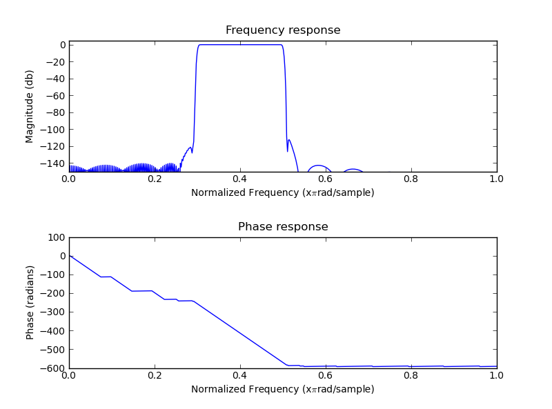
Functions for frequency, phase, impulse and step response
#Plot frequency and phase response
def mfreqz(b,a=1):
    w,h = signal.freqz(b,a)
    h_dB = 20 * log10 (abs(h))
    subplot(211)
    plot(w/max(w),h_dB)
    ylim(-150, 5)
    ylabel('Magnitude (db)')
    xlabel(r'Normalized Frequency (x$\pi$rad/sample)')
    title(r'Frequency response')
    subplot(212)
    h_Phase = unwrap(arctan2(imag(h),real(h)))
    plot(w/max(w),h_Phase)
    ylabel('Phase (radians)')
    xlabel(r'Normalized Frequency (x$\pi$rad/sample)')
    title(r'Phase response')
    subplots_adjust(hspace=0.5)

#Plot step and impulse response
def impz(b,a=1):
    l = len(b)
    impulse = repeat(0.,l); impulse[0] =1.
    x = arange(0,l)
    response = signal.lfilter(b,a,impulse)
    subplot(211)
    stem(x, response)
    ylabel('Amplitude')
    xlabel(r'n (samples)')
    title(r'Impulse response')
    subplot(212)
    step = cumsum(response)
    stem(x, step)
    ylabel('Amplitude')
    xlabel(r'n (samples)')
    title(r'Step response')
    subplots_adjust(hspace=0.5)