Linear Regression Models with Python
Author: Matti Pastell
Tags:
Python, Pweave
Apr 19 2013
I have been looking into using Python for basic statistical analyses lately and I decided to write a short example about fitting linear regression models using statsmodels-library.
Requirements
This example uses statsmodels version 0.5 from github and we’ll use the new formula API which makes fitting the models very familiar for R users. You’ll also need Numpy, Pandas and matplolib.
The analysis has been published using Pweave development version. See my other post.
Import libraries
import pandas as pd
import numpy as np
import statsmodels.formula.api as sm
import matplotlib.pyplot as plt
We’ll use whiteside dataset from R package MASS. You can read the description of the dataset from the link, but in short it contains:
The weekly gas consumption and average external temperature at a house in south-east England for two heating seasons, one of 26 weeks before, and one of 30 weeks after cavity-wall insulation was installed.
Read the data from pydatasets repo using Pandas:
url = 'https://raw.github.com/cpcloud/pydatasets/master/datasets/MASS/whiteside.csv'
whiteside = pd.read_csv(url)
Fitting the model
Let’s see what the relationship between the gas consumption is before the insulation. See statsmodels documentation for more information about the syntax.
model = sm.ols(formula='Gas ~ Temp', data=whiteside, subset = whiteside['Insul']=="Before")
fitted = model.fit()
print fitted.summary()
                            OLS Regression Results
==============================================================================
Dep. Variable:                    Gas   R-squared:                       0.944
Model:                            OLS   Adj. R-squared:                  0.941
Method:                 Least Squares   F-statistic:                     403.1
Date:                Fri, 19 Apr 2013   Prob (F-statistic):           1.64e-16
Time:                        16:07:56   Log-Likelihood:                -2.8783
No. Observations:                  26   AIC:                             9.757
Df Residuals:                      24   BIC:                             12.27
Df Model:                           1
==============================================================================
                 coef    std err          t      P>|t|      [95.0% Conf. Int.]
------------------------------------------------------------------------------
Intercept      6.8538      0.118     57.876      0.000         6.609     7.098
Temp          -0.3932      0.020    -20.078      0.000        -0.434    -0.353
==============================================================================
Omnibus:                        0.296   Durbin-Watson:                   2.420
Prob(Omnibus):                  0.862   Jarque-Bera (JB):                0.164
Skew:                          -0.177   Prob(JB):                        0.921
Kurtosis:                       2.839   Cond. No.                         13.3
==============================================================================
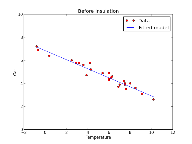
Plot the data and fit
Before = whiteside[whiteside["Insul"] == "Before"]
plt.plot(Before["Temp"], Before["Gas"], 'ro')
plt.plot(Before["Temp"], fitted.fittedvalues, 'b')
plt.legend(['Data', 'Fitted model'])
plt.ylim(0, 10)
plt.xlim(-2, 12)
plt.xlabel('Temperature')
plt.ylabel('Gas')
plt.title('Before Insulation')
Fit diagnostiscs
Statsmodels OLSresults objects contain the usual diagnostic information about the model and you can use the get_influence() method to get more diagnostic information (such as Cook’s distance).
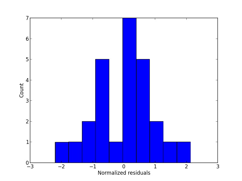
A look at the residuals
Histogram of normalized residuals
plt.hist(fitted.norm_resid())
plt.ylabel('Count')
plt.xlabel('Normalized residuals')
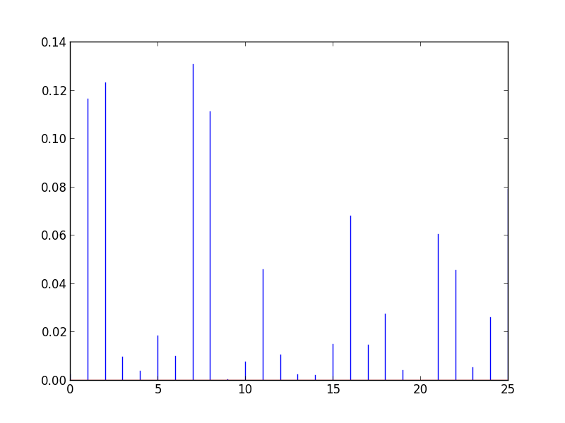
Cooks distance
OLSInfluence objects contain more diagnostic information
influence = fitted.get_influence()
#c is the distance and p is p-value
(c, p) = influence.cooks_distance
plt.stem(np.arange(len(c)), c, markerfmt=",")
Statsmodels builtin plots
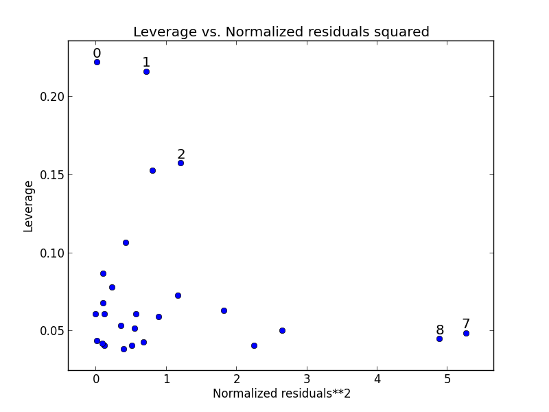
Statsmodels includes a some builtin function for plotting residuals against leverage:
from statsmodels.graphics.regressionplots import *
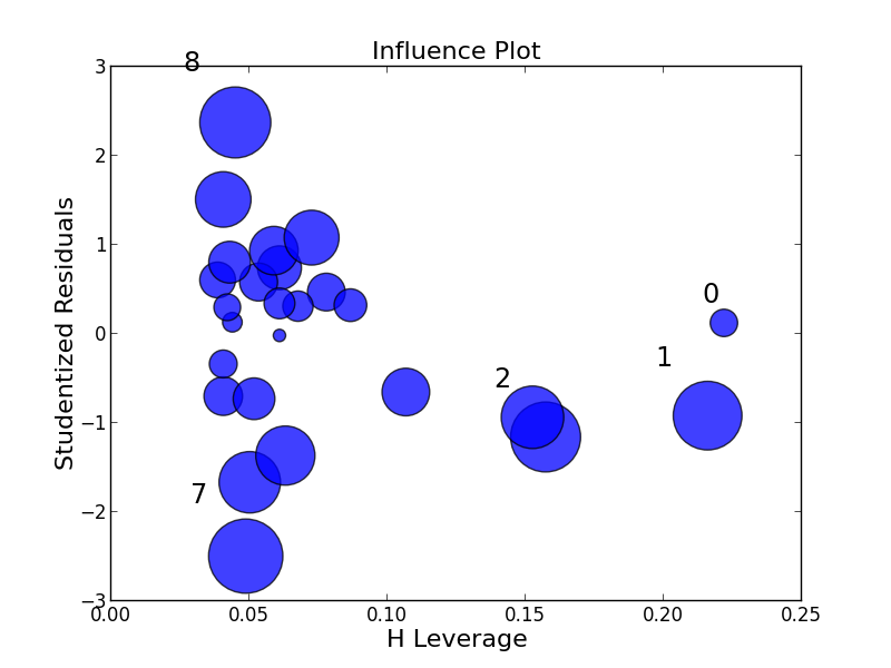
plot_leverage_resid2(fitted)
influence_plot(fitted)