IIR filter design with Python and SciPy
Author: Matti Pastell
Tags:
SciPy, Python, DSP
May 11 2009
I have had some trouble in IIR filter design with SciPy, e.g. getting the filter phase response and impulse response. After some searching and looking at different examples e.g. here I managed to get what I wanted. So here is a simple example on how to make a filter with Scipy, I hope it helps someone else. The example requires Scipy+Numpy+matplolib. You can also download the entire code: elliptic_bandpass.py
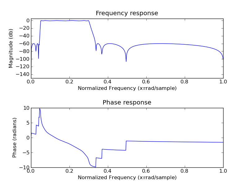
For the desing use scipy.signal.iirdesign function, the following designs an elliptic bandpass filter with passband from 0.05 to 0.3 times the Nyquist frequency with 60 db stop band and 1 db passband attenuation:
from pylab import *
import scipy.signal as signal
b,a = signal.iirdesign(wp = [0.05, 0.3], ws= [0.02, 0.35], gstop= 60, gpass=1, ftype='ellip')
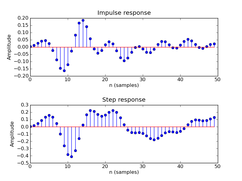
SciPy has a ready made function for calculating the frequency response of the filter, but not for phase, impulse or step response. Thats why I made two Matlab style functions, mfreqz for calculating and plotting frequency and phase response and impz for plotting impulse and step response, the code for the functions is in the end of the post and here is the output:
mfreqz(b, a)
impz(b, a)
And here are the functions I used:
def mfreqz(b,a=1):
    w,h = signal.freqz(b,a)
    h_dB = 20 * log10 (abs(h))
    subplot(211)
    plot(w/max(w),h_dB)
    ylim(-150, 5)
    ylabel('Magnitude (db)')
    xlabel(r'Normalized Frequency (x$\pi$rad/sample)')
    title(r'Frequency response')
    subplot(212)
    h_Phase = unwrap(arctan2(imag(h),real(h)))
    plot(w/max(w),h_Phase)
    ylabel('Phase (radians)')
    xlabel(r'Normalized Frequency (x$\pi$rad/sample)')
    title(r'Phase response')
    subplots_adjust(hspace=0.5)
    show()

def impz(b,a=1):
    impulse = repeat(0.,50); impulse[0] =1.
    x = arange(0,50)
    response = signal.lfilter(b,a,impulse)
    subplot(211)
    stem(x, response)
    ylabel('Amplitude')
    xlabel(r'n (samples)')
    title(r'Impulse response')
    subplot(212)
    step = cumsum(response)
    stem(x, step)
    ylabel('Amplitude')
    xlabel(r'n (samples)')
    title(r'Step response')
    subplots_adjust(hspace=0.5)
    show()